Linear Regression
Used to predict one continuous variable from another continuous variable.
Slope: The change in the Y variable depending on an change in the X variable.
\(b_{1}\) = r(\(\displaystyle \frac{\ sd (Y)}{\ sd (X)}\))
Correlation between the standard deviation of Y and the standard deviation of X.
Intercept: The point of intersection between the regression line and the y axis when the X variable is 0.
\(b_{0}\) = \(\overline{Y}\) - \(b_{1}\) * \(\overline{X}\)
Subtracting mean of X variable times slope from the mean of Y variable.
library(dplyr)
library(tidyr)
library(broom)
library(ggplot2)
library(ggridges)
library(ggfortify)
library(extremevalues)
library(reactable)
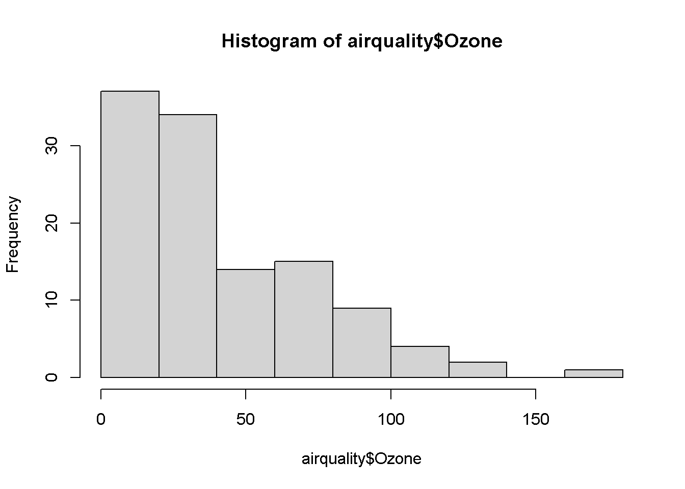
hist(airquality$Ozone)
Square root of the ozone variable because it is right skewed.
airquality_sqrt <- airquality %>% filter(!is.na(Ozone))

airquality_sqrt$Ozone <- sqrt(airquality_sqrt$Ozone)
airquality_sqrt <- airquality_sqrt[-82,] #this was one outlier
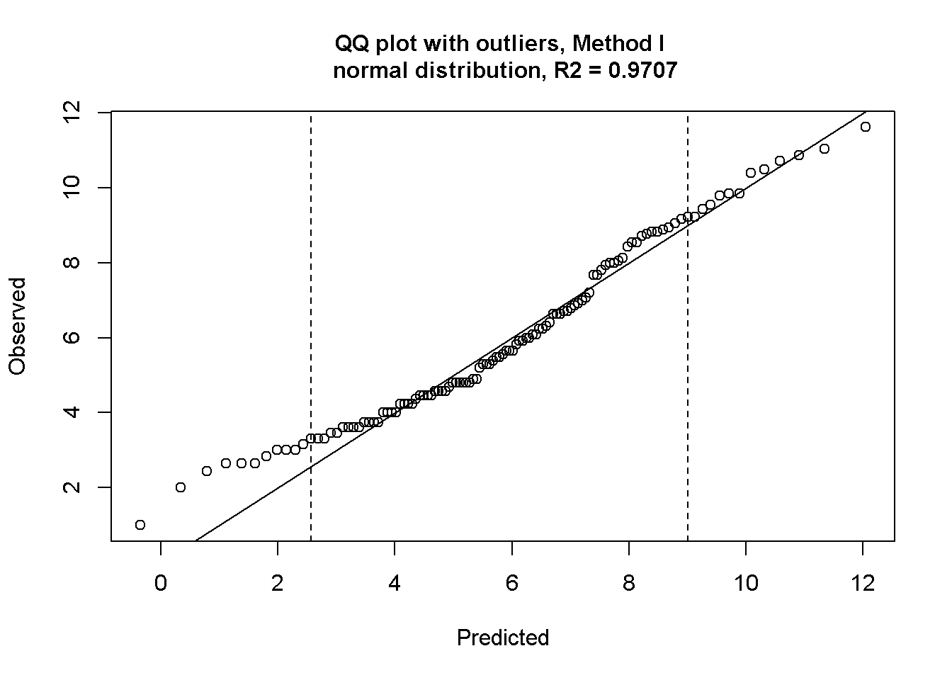
Checking normality and outliers
outlierPlot(airquality_sqrt$Ozone, getOutliers(airquality_sqrt$Ozone))
Data looks workable now.
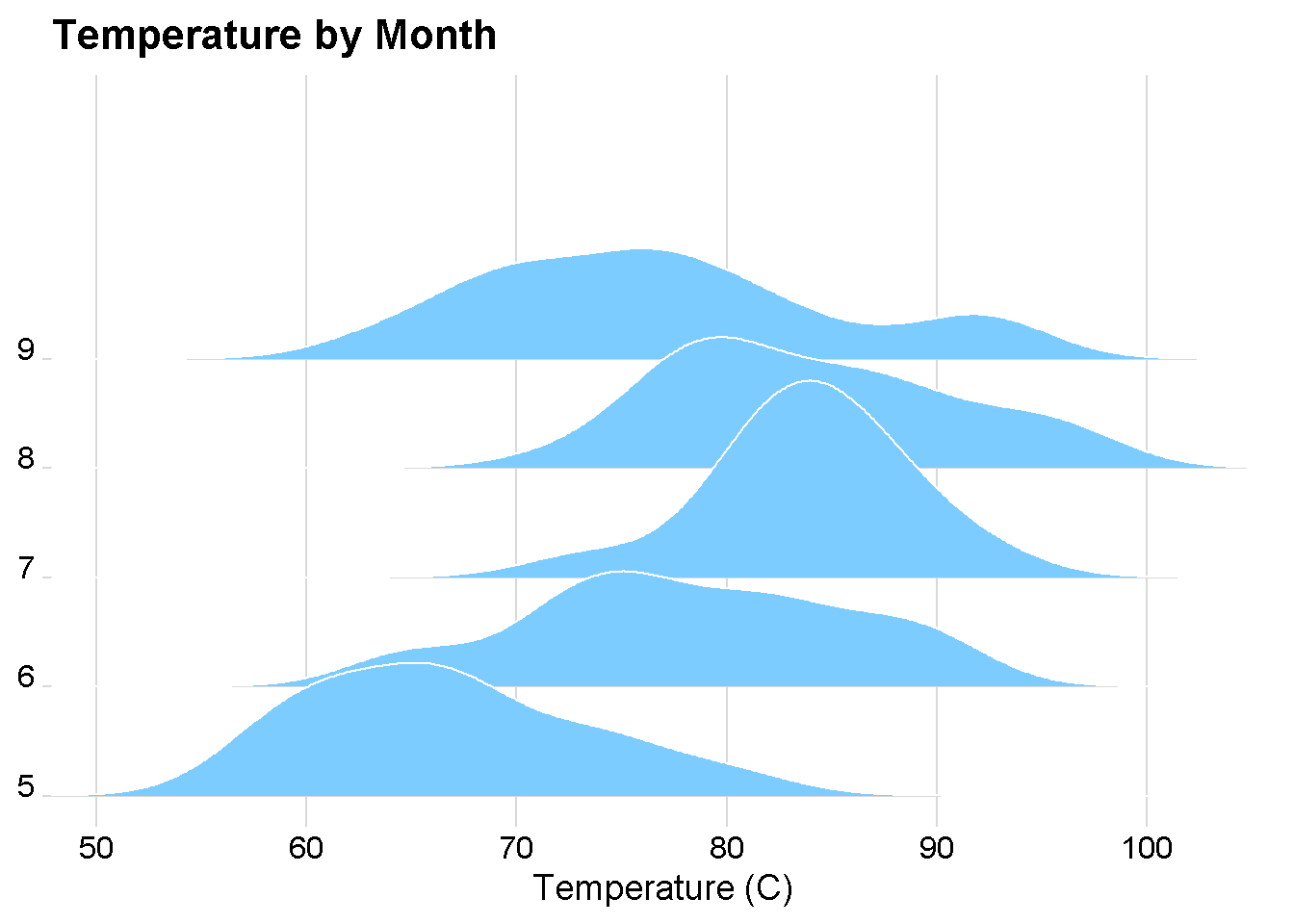
ggplot(airquality_sqrt) +
  aes(x = Temp, y = as.factor(Month)) +
  geom_density_ridges(fill = "#7DCCFF", color = "white") +
  cowplot::theme_minimal_grid() +
  theme(axis.text.y = element_text(vjust = 0)) +
  scale_x_continuous(name = "Temperature (C)",
                     expand = c(0, 0)) +
  scale_y_discrete(name = NULL,
                   expand = expansion(add = c(0.2, 2.6))) +
  labs(title = "Temperature by Month")
model <- lm(Temp ~ Ozone, data = airquality_sqrt)

summary(model)
##
## Call:
## lm(formula = Temp ~ Ozone, data = airquality_sqrt)
##
## Residuals:
## Min 1Q Median 3Q Max
## -15.899 -4.244 1.230 4.069 12.406
##
## Coefficients:
## Estimate Std. Error t value Pr(>|t|)
## (Intercept) 59.418 1.576 37.70 <2e-16 ***
## Ozone 3.090 0.246 12.56 <2e-16 ***
## ---
## Signif. codes: 0 '***' 0.001 '**' 0.01 '*' 0.05 '.' 0.1 ' ' 1
##
## Residual standard error: 6.179 on 113 degrees of freedom
## Multiple R-squared: 0.5827, Adjusted R-squared: 0.579
## F-statistic: 157.8 on 1 and 113 DF, p-value: < 2.2e-16Sigma stands for standard residual error. It is calculated by taking the sum of squared residual values in a model and dividing it by degrees of freedom (# of observations - model coefficients) and taking the square root of that number. SRE is the typical difference between the actual values and the predicted values.
Another metric is the root-mean-square error: it is the same thing with RSE but instead of dividing the sum of squared residuals with degrees of freedom, we simply divide it by the number of observations. It still quantifies the inaccuracy of the model but RMSE is slightly worse than RSE.
We can specifically get the RSE with the pull() function in dpylr after the glance() in broom.
model %>%
  glance() %>%
  pull(sigma)
## [1] 6.178574Leverage (Hat values)
Leverage: how extreme the explanatory variables are. They are called “hatvalues”
In the augment() function, we can see the leverage in the “.hat” column
model %>%
  augment() %>%
  reactable(compact = T, highlight = T, striped = T,
            defaultColDef = colDef(
              format = colFormat(separators = T, digits = 3)))
Influence
A “leave one out” metric: How much the data would change without that data point. The influence of each observation point is based on the size of the residuals and the leverage. This is called “Cook’s distance.” Bigger the Cook’s distance, bigger the influence. We can see it in the augment() function again.
model %>%
  augment() %>%
  arrange(desc(.cooksd)) %>%
  reactable(compact = T, striped = T,
            defaultColDef = colDef(
              format = colFormat(separators = T, digits = 3)))
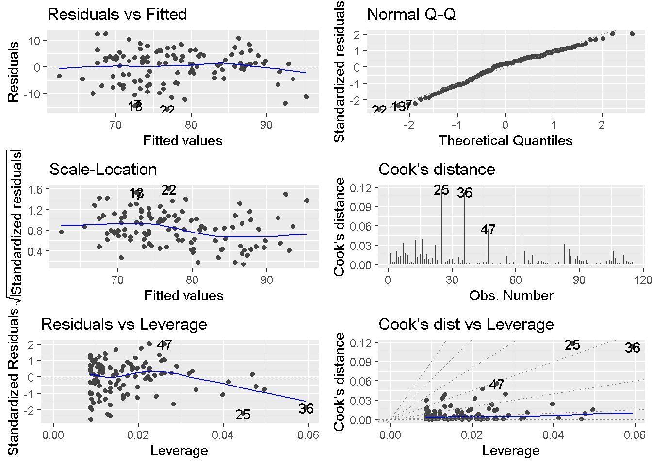
We can see the diagnostic plots by autoplot() function.
autoplot(model, which = 1:6,
         nrow = 3, ncol = 2)
