In this notebook, we will be conducting an ANCOVA analysis for the effects of different exercise regiments on stress levels, controlling for age.
knitr::opts_chunk$set(message=FALSE)
knitr::opts_chunk$set(warning=FALSE)

library(dplyr) #(for data handling)
library(car); #(for Levene test, Type III sums of squares)
library(compute.es) #(for effect sizes)
library(effects) #(for adjusted means)
library(ggplot2)  #(for graphs)
library(ggpubr) #(for advanced graphs)
library(multcomp) #(for post hoc tests)
library(pastecs) #(for descriptive statistics)
library(performance) #(for model peformance evaluation)
library(flextable) #(for tables)
library(see) #(for more plots)
The main premise of ANCOVA is checking the effect of 3 or more independent variables on a dependent variable, after controlling for a covariate. A covariate is a variable that explains some of the variance that we couldn’t with our model. That means a covariate must be something that is not related with our independent variables, but it must be related to the measure we are trying to assess (predicted). After controlling for the covarite, we are able to explain more of the variance in totality of the experiment.
Let’s say that we are looking for the changes in stress levels for different levels of exercise regiments; a low, a moderate and a high level of exercise. Additionally, we want to control for age of the participants for we know that some studies suggests that stress increases with age.
stress <- datarium::stress

stress$exercise <- factor(stress$exercise,
                          labels = c("low", "moderate", "high"), ordered = T)

skimr::skim(stress)| Name | stress |
| Number of rows | 60 |
| Number of columns | 5 |
| _______________________ | |
| Column type frequency: | |
| factor | 2 |
| numeric | 3 |
| ________________________ | |
| Group variables | None |
Variable type: factor
| skim_variable | n_missing | complete_rate | ordered | n_unique | top_counts |
|---|---|---|---|---|---|
| treatment | 0 | 1 | FALSE | 2 | yes: 30, no: 30 |
| exercise | 0 | 1 | TRUE | 3 | low: 20, mod: 20, hig: 20 |
Variable type: numeric
| skim_variable | n_missing | complete_rate | mean | sd | p0 | p25 | p50 | p75 | p100 | hist |
|---|---|---|---|---|---|---|---|---|---|---|
| id | 0 | 1 | 30.50 | 17.46 | 1.0 | 15.75 | 30.50 | 45.25 | 60 | ▇▇▇▇▇ |
| score | 0 | 1 | 84.58 | 8.12 | 65.8 | 80.40 | 85.55 | 90.80 | 100 | ▃▂▇▇▃ |
| age | 0 | 1 | 59.95 | 4.36 | 52.0 | 57.00 | 60.00 | 62.00 | 75 | ▃▇▃▁▁ |
Analyzing data and Checking assumptions
We will do an ANCOVA analysis for the effects of exercise on stress levels, controlling for age.
Outliers
plot(check_outliers(stress$score, method = "iqr"))
It seems that we don’t have any outliers for the stress variable.
Mean stress scores
stress %>%
  group_by(exercise) %>%
summarise(mean_stress = mean(score)) %>% flextable() %>% theme_tron()exercise | mean_stress |
low | 88.725 |
moderate | 88.115 |
high | 76.890 |
It seems that the higher exercise group has lower stress levels, compared to other two groups.
ggviolin(stress, "exercise", "score",  color = "darkblue",
         add = "boxplot", add.params = list(fill = "exercise")) +
  theme(legend.position = "right")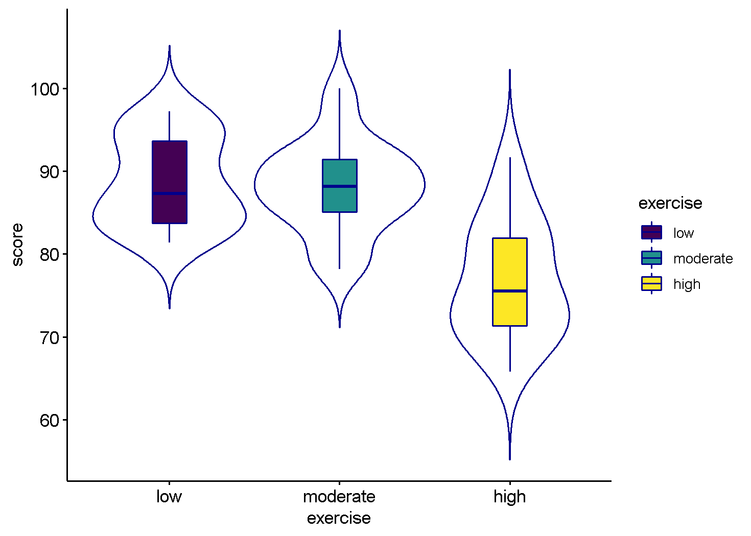
Now, lets look at some descriptive statistics.
by(stress$score, stress$exercise, stat.desc, basic = F, norm = T) ## stress$exercise: low
## median mean SE.mean CI.mean.0.95 var std.dev
## 87.30000000 88.72500000 1.20564189 2.52343748 29.07144737 5.39179445
## coef.var skewness skew.2SE kurtosis kurt.2SE normtest.W
## 0.06076973 0.22965819 0.22423032 -1.56191082 -0.78694912 0.91222171
## normtest.p
## 0.07027058
## ------------------------------------------------------------
## stress$exercise: moderate
## median mean SE.mean CI.mean.0.95 var std.dev
## 88.15000000 88.11500000 1.24567198 2.60722142 31.03397368 5.57081445
## coef.var skewness skew.2SE kurtosis kurt.2SE normtest.W
## 0.06322209 0.10287876 0.10044727 -0.46414885 -0.23385556 0.97765929
## normtest.p
## 0.90042914
## ------------------------------------------------------------
## stress$exercise: high
## median mean SE.mean CI.mean.0.95 var std.dev
## 75.50000000 76.89000000 1.59769406 3.34401210 51.05252632 7.14510506
## coef.var skewness skew.2SE kurtosis kurt.2SE normtest.W
## 0.09292632 0.40388522 0.39433957 -0.97258818 -0.49002632 0.95476368
## normtest.p
## 0.44520271By the look of skew.2SE and kurt.2SE values, data doesn’t seem skewed or kurtosed.
Levene’s test for homogeniety of variances
leveneTest(stress$score, stress$exercise, center = mean) %>% flextable() %>% theme_tron()Df | F value | Pr(>F) |
2 | 1.565691 | 0.2177959 |
57 |
The p value is not significant so we can assume variances are homogeneous; we can continue with our model.
Homogeneity of regression slopes
It’s time to check the assumption of homogeneity of regression slopes. This assumption basically assumes that the relationship between the covariate (age) and outcome variable (anxiety scores) should be similar at different levels of the predictor variable (exercise groups). To test this, we need to conduct ANCOVA just like the actual model but with an addition; including the interaction between the IV’s (exercise groups) and the covariate (age).
hrs_model <- aov(score ~ exercise + age + exercise:age, data = stress)

Anova(hrs_model, type = "III")
## Anova Table (Type III tests)
##
## Response: score
## Sum Sq Df F value Pr(>F)
## (Intercept) 529.64 1 15.8904 0.000203 ***
## exercise 21.05 2 0.3158 0.730555
## age 261.19 1 7.8363 0.007087 **
## exercise:age 13.70 2 0.2055 0.814867
## Residuals 1799.88 54
## ---
## Signif. codes: 0 '***' 0.001 '**' 0.01 '*' 0.05 '.' 0.1 ' ' 1The assumption can be checked with the p value of the interaction: exercise:age. Since it is not significant, we can say that the regression slopes are the same for different levels of the predictor variable; assumption is not violated and we can continue with our actual model.
stress %>%
  ggplot(aes(age, score)) +
  geom_point() +
  geom_smooth(method = "lm", se = F,
              aes(color = exercise)) +
  ylab("Stress Score") +
  xlab("Age")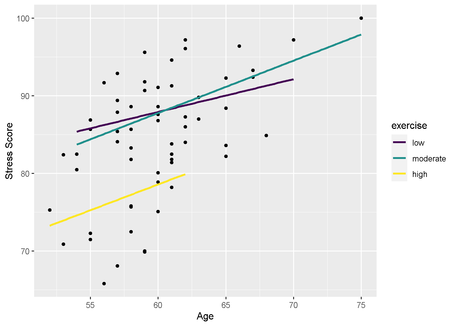
ANCOVA Model
Lets start building the model. First we set up an orthogonal contrast such that we compare high exercise group with other groups. In our model, we want to compare low & moderate to high first, then compare low to moderate. The rule with the contrasts is that you code them in a way that the total in that contrast will amount to 0 while the groups to be contrasted will be opposite to each other.
contrasts(stress$exercise) <- cbind(c(1, 1,-2), c(-1,1,0))Then we build the model
anc_model <- aov(score ~ age + exercise, data = stress)
# we'll apply type III, so order does not matter
Diagnostics of the model
Before we go on to analyze our model, we’ll look into some diagnostics and assumptions of the model.
check_model(anc_model)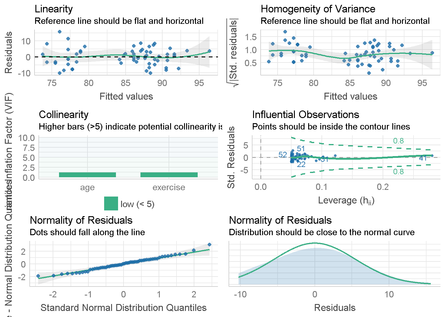
It seems out model is a perfect fit (well, almost). The only somewhat troubled assumption seems to be in the heteroscedasticity (homogeneity of variances) but we did a levene test before, and it was not significant. So, I say we are good to continue.
model_performance(anc_model) %>% flextable() %>% theme_tron()AIC | BIC | R2 | R2_adjusted | RMSE | Sigma |
384.7954 | 395.2671 | 0.5335764 | 0.5085894 | 5.497848 | 5.690813 |
Model Analysis
Finally, we’ll analyze the model with type III sums of squares.
Anova(anc_model, type = "III")## Anova Table (Type III tests)
##
## Response: score
## Sum Sq Df F value Pr(>F)
## (Intercept) 640.96 1 19.7917 4.151e-05 ***
## age 298.42 1 9.2147 0.003639 **
## exercise 980.91 2 15.1444 5.528e-06 ***
## Residuals 1813.58 56
## ---
## Signif. codes: 0 '***' 0.001 '**' 0.01 '*' 0.05 '.' 0.1 ' ' 1Intercept is not particularly important; It shows the model when all the other variables are 0, therefore it doesn’t have a meaning in this study. From the age response, we can see that our covariate (age) significantly predicts stress (p = 0.003639). Therefore, we can conclude that people’s stress levels are influenced by their age. Furthermore, after controlling for the effects of age, exercise regiments highly significantly influence stress levels. However, we just can’t look at their means to find out which exercise groups differ; we have to look at the adjusted means (adjusted for age) to accurately interpret the differences.
adjustedAnc <- effect("exercise", anc_model, se = T) # se stands for standard error

adjustdf <- as.data.frame(adjustedAnc)
adjustdf$exercise <- factor(adjustdf$exercise,
                            levels = c("low", "moderate", "high"),
                            ordered = T)

adjustdf %>% flextable() %>% theme_tron()exercise | fit | se | lower | upper |
low | 87.61061 | 1.324401 | 84.95752 | 90.26371 |
moderate | 87.80069 | 1.276710 | 85.24313 | 90.35824 |
high | 78.31870 | 1.356754 | 75.60080 | 81.03661 |
We can see that high exercise group has the lowest anxiety scores while low and moderate exercise groups have the highest. Let’s visualize that.
adjustdf %>%
  ggplot(aes(exercise, fit)) +
  geom_errorbar(aes(ymin = fit-se, ymax = fit+se),
                color = "red", width = .3) +
  geom_point() +
  theme_lucid() +
  labs(title = "Adjusted stress means for exercise regiments") +
  ylab("Stress Score") +
  xlab("Exercise")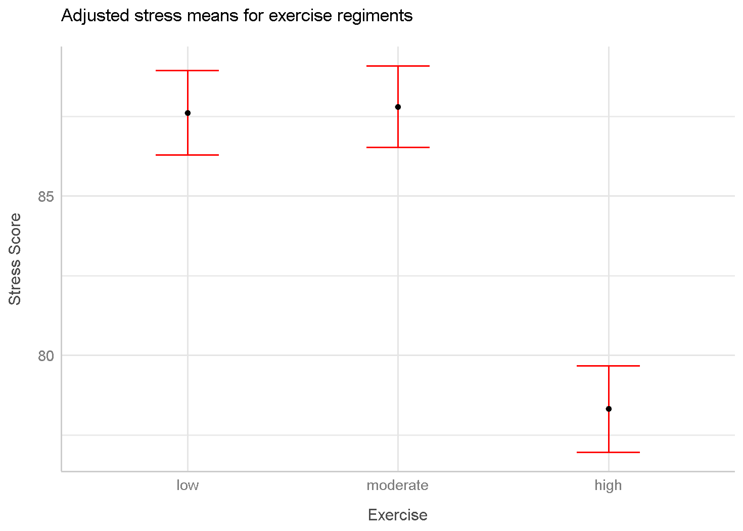
Planned contrasts
Okay, it’s time to analyze our contrasts.
summary.lm(anc_model) ##
## Call:
## aov(formula = score ~ age + exercise, data = stress)
##
## Residuals:
## Min 1Q Median 3Q Max
## -10.2614 -3.5603 0.1086 3.5856 15.6386
##
## Coefficients:
## Estimate Std. Error t value Pr(>|t|)
## (Intercept) 50.31643 11.31014 4.449 4.15e-05 ***
## age 0.57148 0.18826 3.036 0.00364 **
## exercise1 3.12898 0.57031 5.486 1.02e-06 ***
## exercise2 0.09504 0.90940 0.105 0.91714
## ---
## Signif. codes: 0 '***' 0.001 '**' 0.01 '*' 0.05 '.' 0.1 ' ' 1
##
## Residual standard error: 5.691 on 56 degrees of freedom
## Multiple R-squared: 0.5336, Adjusted R-squared: 0.5086
## F-statistic: 21.35 on 3 and 56 DF, p-value: 2.386e-09Age is significantly influencing the stress levels, as we have seen previously. The interesting point here is the b-value (Estimate) which is .57. This means that for every ~.6 years in age, stress levels increase by 1.
Exercise1 compares the adjusted mean for the high group on one side and the mean of adjusted means of the moderate-low groups on the other. We can clearly see that the high exercise group is significantly different from other two groups when influencing stress levels. Therefore the b-value (Estimate) is (((87.61061 + 87.80069)/2) - 78.31870)/3 = 3.12898. The value is divided by the number of groups within the contrasts we did in exercise1 (3).
Exercise2 compares the difference between the adjusted means for moderate and the low exercise groups, so the b-value is (87.80069 - 87.61061)/2 = 0.09504. The value, again, is divided by the number of contrasts in that comparison (high and low). The t statistic is not significant, so as we can tell, low and moderate exercise groups do not differ in their effect on the stress levels.
Post hoc Test
Since we want to test adjusted means, we need to use the glht() function; pairwise.t.test() function will not test the adjusted means. Likewise, we can only use Tukey or Dunnett’s post hoc tests.
posthoc <- glht(anc_model, linfct = mcp(exercise = "Tukey"))

summary(posthoc)
##
## Simultaneous Tests for General Linear Hypotheses
##
## Multiple Comparisons of Means: Tukey Contrasts
##
##
## Fit: aov(formula = score ~ age + exercise, data = stress)
##
## Linear Hypotheses:
## Estimate Std. Error t value Pr(>|t|)
## moderate - low == 0 0.1901 1.8188 0.105 0.994
## high - low == 0 -9.2919 1.9850 -4.681 <1e-04 ***
## high - moderate == 0 -9.4820 1.8890 -5.020 <1e-04 ***
## ---
## Signif. codes: 0 '***' 0.001 '**' 0.01 '*' 0.05 '.' 0.1 ' ' 1
## (Adjusted p values reported -- single-step method)As we have suspected, high exercise group significantly differs from the moderate, as well as the low exercise group.
- (Moderate - low) 87.80069 - 87.61061 = 0.1901
- (High - low) 78.31870 - 87.61061 = -9.2919
- (High - moderate) 78.31870 - 87.80069 = -9.4820
The t values are just the estimate values (adjusted mean differences) divided by standard error.
Confidence intervals
Lastly, we can check the confidence intervals for the post hoc analysis.
confint(posthoc)##
## Simultaneous Confidence Intervals
##
## Multiple Comparisons of Means: Tukey Contrasts
##
##
## Fit: aov(formula = score ~ age + exercise, data = stress)
##
## Quantile = 2.4072
## 95% family-wise confidence level
##
##
## Linear Hypotheses:
## Estimate lwr upr
## moderate - low == 0 0.1901 -4.1881 4.5683
## high - low == 0 -9.2919 -14.0703 -4.5135
## high - moderate == 0 -9.4820 -14.0292 -4.9348Another metric to look in confidence intervals is whether the lower and the upper intervals cross 0; if they do, it means that the true difference between group means might be 0, therefore no difference. This is the case only in the high and moderate exercise groups, as expected.
